
| What is | |
The Object Watershed Link Simulation (OWLS) Program is designed to physically and visually simulate the real time or short-term hydrological processes for small forested watersheds and to provide detailed information about watershed response to environmental changes.
In order to attain the objective of this study, the design of the OWLS model employed a programming method more sophisticated than commonly used programming methods (e.g., FORTRAN programming). The Object Orientation Programming (OOP) Method (coded using C++) was used to construct the OWLS model. In OOP, an object is defined as a container of data type (or class in C++) which has some specific properties or features (or data members) and which also has certain types of functions (also called member functions). The philosophy of the OOP method is understandable if you consider the relation between cells and the human body: In order to understand the functionality of the human body, a doctor needs to know how many different kinds of cells a human has, what is in them, and how they function and relate to other cells. In addition, he/she needs to know how they are organized to form the organs and finally how the organ functions in the human body.
The OOP method used for watershed simulation is based on a similar philosophy: Starting from the basic components (objects) of the watershed(i.e., points, lines and cells), the properties that these objects have (e.g., elevation, length, slope, soil, vegetation ...) and the types of functions they perform (e.g., infiltration, surface flow ...) are established. Then, the relations between these objects (linkage) to form the "organs" of the watershed (e.g., flow path, stream network, canopy, surface, soil, macropore pipes ...) are specified. Finally, it is necessary to establish how these "organs" operate together (linkage) to reflect watershed behavior (e.g., streamflow, stream chemistry).
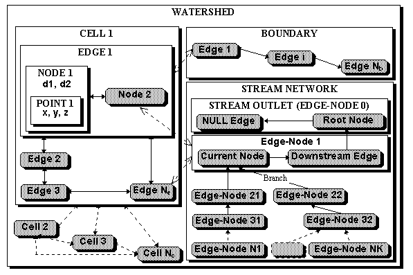
Within the OWLS model, there are numerous objects representing many different components of a watershed. Following table includes the selected objects used in OWLS; a complete list of objects is included in Appendix I from technical documents.
| OWLS Modules | Object Name (Induced Object) | Descriptions | Features (Additional Features) | Functions (Additional Functions) |
| OWLSFacet | OWLSFacet | object for facet | *parent [OWLSPolyhedron] nNodes *nodeIdxs color [Color] area |
draw fill unitNormalMC unitNormalWC facetColor getFacetArea whichSide intersect reflect |
| OWLSCell | cell object for watershed model | (*parent) [OWLSWatershed] (marked) (nEdges) (*edgesIdx) (*edgesWeight) (value) (info) [sCellInfo] |
(save) (read) (print) (getCellInfo) (getWeight) (nodeInCell) (nodeOnCell) (getCellArea) (averageAspect) (unitNormalMC) |
|
| OWLSPoint | OWLSPoint | point object | x y z w |
operator + operator - operator * |
| OWLSGauge | gauge object for watershed | (name) (dataFile) (nRecords) (startTime)[OWLSTime] (endTime)[OWLSTime] (step) |
||
| OWLSNode | node object for watershed model | (d1) (d2) |
(save) (read) |
In the table above, OWLSFacet and OWLSPoint are object modules; each is a stand-alone object group within the model. There are many "induced" objects, for example, OWLSCell is induced from the OWLSFacet (a geometric object) and represents the unit area for watershed model. The OWLSCell is not only a geometric object, but also a watershed object with the additional features like weights for the edges, value for the cell, relations (pointers) to other watershed objects and functions like save, read, getWeight, etc. Similarly, the OWLSNode is a point object for watershed model with the addition of soil depths (d1, d2 for two layers) and functions. The OWLSGauge is a watershed object for gauge stations (i.e., water gauge, rain gauge, and air temperature gauge). It has a name, time range, etc., which its parent object (OWLSPoint) does not include.
In the OWLS program, objects are linked in basically three formats. Table 1 - 2 demonstrates the examples of these formats.
| Main Object | Internal Linked Object | Inherited Linked Objects | External Linked Objects |
| OWLSWatershed | OWLSObject |
OWLSNode OWLSEdge OWLSCell OWLSenTree OWLSBiTree OWLSPath OWLSPathNode | |
| OWLSHydrology |
OWLSFlow OWLSCloud | OWLSWatershed |
OWLSRain OWLSTemp OWLSGauge OWLSSoil OWLSVegetation |
| OWLSStream |
OWLSWatershed OWLSSegment OWLSStream |
(1) Internal linkage: One object is included within another. For example, the object OWLSFlow is included within object OWLSHydrology. It becomes one of the features of OWLSHydrology. When the object of OWLSHydrology is called in the OWLS model, its internal object OWLSFlow will be called automatically. Features of OWLSFlow are automatically transferred to OWLSHydrology (in-to-out linkage).
(2) Inherited linkage: One object is "inherited" from another object. For example, the object OWLSHydrology is the inherited object from OWLSWatershed, which is also inherited from the general OWLS object OWLSObject. Parameters (features) of OWLSWatershed will automatically pass to OWLSHydrology (parent-to-children linkage).
(3) External linkage: One object contains a member acting as a gateway to another object. Such a member is also called a pointer, or an External linkage in OWLS' terminology. In such cases, some functions of the object can use parameters from another object through this linkage without complex analytic procedures. External linkage not only makes the cell-to-cell connection possible and is accomplished relatively easily, but also assists in the connection of flow paths and stream networks in the OWLS model.
A complete list of the linkages in the OWLS model is included in Appendix II.
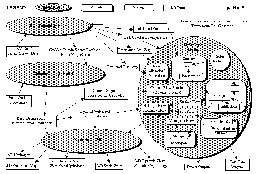
The OWLS model is comprised of four primary models (or sub-models) (See the Figure below). The Data Processing Model is a set of modules handling the conversion of raw data into OWLS' data format. The Geomorphologic Model is the combination of several modules, including a data conversion module which converts topographical data into 3-D vector data, a flowpath module to delineate catchment boundary, flow path and stream network, and so on. The Hydrologic Model is a group of modules simulating different hydrological aspects in the watershed processes, including a precipitation model, an interception model, a solar radiation model, an infiltration model, an evaportranspiration model, a macropore model, a surface water routing model, a soil water routing model, a channel water routing model, and so on. The Visualization Model is a group of modules whose functions are to display the digital data format onto a computer screen or as a printout. The OWLS 3-D visualization model is used to develop a three dimensional view of the watershed.
 |
The Object Watershed Link System (OWLS) is a physically-based hydrologic model. The following characterizations identify its main features relative to other watershed models. A conclusion is listed in a seperated table.
1. It is coded in C++ object orientated programming (OOP), containing modules and codes that are reusable and expandable. Also, it utilizes a dynamic memory allocation mechanism to reduce the usage of computer memory when running. This makes it possible to run a large program in a personal computer. In addition, the object-orientated programming makes the platform independent graphic interface (PIGI) possible in the OWLS, which provides great potential for the future development of the model.
2. It is structured as objects and linkages; all watershed components, hydrologic components, and even time and measurement units are represented as objects and are linked with each other. Each object not only identifies itself from others, but also carries characteristic data to wherever it goes. It provides a higher efficiency for running the model.
3. Automatic watershed delineation is vector-based. It identifies the watershed boundary, possible stream channel, and their hydrologic characteristics. It provides a harmonious simulation base for the hydrologic model.
4. The OWLS model is a vector-based and true 3-D hydrologic simulation model. A watershed is a linkage of three dimensional cells, edges and nodes. Thus, hydrologic components are nested into these 3-D cells, edges and nodes; thus, the hydrologic processes become a dynamic linkage among them.
5. The OWLS model is designed to handle any kind of cell geometry or their combination in terms of watershed topography or hydrology. Because of the OOP and dynamic memory management, the OWLS model defines the object of a cell having undetermined numbers of nodes and edges; this can be accomplished while data are being input. Therefore, each cell of a watershed can be a triangle, a rectangle, or an x-edges polygon, there are no restriction on cell characteristics. To handle different cell geometries, the Equivalent-Rectangle Simplification (ERS) procedure unifies all cells by finding a hydrological equivalent-rectangle for each and calculates the weights for each edges.
6. The hydrologic model is constructed over the 3-D watershed, from each cell, to each segment of the potential stream. In the vertical dimension, there are three and half layers: the canopy layer, the surface layer, the soil layer and the half -- macropore pipe layer, which is nested into the soil layer and invisible. Hydrologic processes considered in the OWLS model includes:
(2) Evaporation: in canopy and surface layer, defined as water vaporized from the water surface of the related layer, calculated from solar radiation, air temperature, and canopy coverage.
(3) Transpiration: in canopy and soil layer, defined as water vaporized from the layer itself. Calculated from potential Evaporation plus the restriction from the available soil moisture and the soil water supply capacity.
(4) Snow melting: in canopy and surface layer, calculated from the simple degree-day function. No energy budget has been taken into account.
(5) Infiltration: in surface layer, calculated by modified Horton’s equation with relative soil moisture content to define the Hortonean time.
(6) Macropore surface water entry: in surface layer, calculated as proportional to infiltration.
(7) Macropore soil water entry: in soil layer, calculated as a function of soil water depth and the relative soil moisture content.
(8) Surface overland flow: calculated by the kinematic wave finite-difference approximation using Manning’s equation.
(9) Subsurface flow in the soil: calculated by the kinematic wave finite-difference approximation using Darcy’s equation.
(10) Macropore flow of the macropore pipe system in the soil: calculated by multiple-pipe finite-difference approximation derived from the energy balance equation;
(11) Hillslope flow routing: all horizontal flows including surface, subsurface and macropore flow are routed by utilizing the edge weights calculated from the ERS method in combination with the kinematic wave finite differential calculations. A three-dimensional routing has been converted into a virtually 1-D flow routing procedure. This technique dramatically reduces the complexity of the flow routing model and increases the flexibility of the model as well as the calculation speed.
(12) Stream flow routing: since information about the stream segments has been calculated from the automatic watershed delineation model and the stream geometric model, the kinematic wave method has been utilized for channel flow routing.
8. The simulation results from the OWLS model not only provided valuable information about the sources of flow generation from a watershed, but also dynamically visualized the concept of Variable Source Area (VSA) from a watershed in a three dimensional aspect. Source area concept in the OWLS model has been expanded: Flow not only comes from the surface of riparian cells, but also from soil macropore and soil matrix.
9. Tremendous amounts of distributed-and-dynamic flow data generated from the OWLS model provide a strong fundation for applications in other fields of studies. For example, by setting the pollution source in the watershed, one can calculate the transportation of the pollutants in the watershed using the data from the OWLS model.
Future development for improving the OWLS model should include the following aspects:
(1) Model testing by applying the OWLS model in other watershed areas. More applications should bring model coefficients closer to reality; more testing could discover unforseen problems (or bugs) currently embedded in the model;
(2) Laboratory testing and field survey to support, verify, modify ,or even rewrite the theories, assumptions, and equations that have been developed and used in the OWLS model. The model has approached many uncertain areas in the hydrology field. Additional data from the field or lab testing will able to enhance the model;
(3) Extending the application of the OWLS model to include watershed sedimentation, water chemistry and pollution processes;
(4) Adding additional features into the stream channel model simulating in-stream woody debris so that it can be used to address more complicated problems for stream ecology;
(5) Expanding the model into different area, e.g. agriculture fields, roads, and urban areas.
(6) Improving the User Interface of the OWLS model so that it can be easier to use.